Modeling
Orbital Debris Problems
|
Overview In this lesson, students
examine the problem of space pollution caused by human-made debris in orbit
to develop an understanding of functions and modeling. It allows the students
an opportunity to use spreadsheets, graphing calculators, and computer
graphing utilities. TEKS:
B1(B) In solving problems, the student
collects data and records results, organizes the data, makes scatterplots,
fits the curves to the appropriate parent function, interprets the results, and
proceeds to model, predict, and make decisions and critical judgments.
C1 (A) The student identifies and sketches
graphs of parent functions, including linear (y = x), quadratic (y = x2),
square root (y = Ö x), inverse (y = 1/x), exponential (y = ax), and
logarithmic (y = logax) functions.
D1 (B) The student relates representations
of quadratic functions, such as algebraic, tabular, graphical, and verbal
descriptions.
F (5) The student analyzes a situation
modeled by an exponential function, formulates an equation or inequality, and
solves the problem.
Objectives
Students will
be able to:
Materials
Instructional
Plan
The
problem of space pollution caused by human-made debris in orbit is presented
as a context for studying mathematical modeling. This unit should help
students realize that not all problems are solvable with precise measurements
and exact answers but that mathematical models enable us to look at trends
and to make predictions about probable outcomes. The ambiguity of some of
these activities may be frustrating to a few students, but it reflects the
realities with which mathematicians and scientists must work. Purposes In
this unit, students create and compare various mathematical models as a way
to investigate some of the questions raised by the proliferation of orbital
debris. Although the models are greatly simplified to make them
understandable to high school students, they offer insight into the process
of mathematical modeling and its importance. Throughout the unit it is
assumed that your students will work with appropriate technology. Depending
on what you have available and what you prefer, these tools may include
graphing calculators, computer graphing utilities, spreadsheets, or
non-graphing calculators. Introduction “One
important outcome for this unit is helping students develop an appreciation
of the power and limitations of mathematical modeling. They should realize
that the two most basic expectations of models are (1) the ability to account
for or represent known phenomena and (2) the ability to predict future
results. Thus, with the models that students develop in this unit, they
should continually be asking such questions as, What will happen if this
trend continues? Or What if this element is change? Other
outcomes that we anticipate from this unit are a better understanding of the
difference among linear, quadratic, and exponential functions (models) and
the patterns of growth that arise from them; a more concrete realization of
the vastness of space and the seeming paradox of having very large quantities
of debris in orbit yet, at the same time, quite small probabilities of
encountering any - although with potentially lethal results should an
encounter happen; and an appreciation of the power of mathematics to help us
"get our arms around " seemingly unmanageable problems. Data
included in this unit are taken from various NASA sources, but you will want
to be alert to updated information and current events related to the problem.
For example, three events in early 1996 received extensive coverage in the
media. One was the Space Shuttle Endeavour's maneuver to steer clear of a
defunct satellite. A second was the breaking loose of a satellite and its
12-mile-long tether during an attempt to deploy it from the Shuttle. A third
was the return to Earth of a Chinese satellite, which problem landed
somewhere in the Background
and Supporting Information “In
January 1996, two days into their mission, the crew of the Space Shuttle
Endeavour performed a maneuver to slow its speed by 4 feet per second,
thereby steering clear of a 350-pound piece of "space junk," a
defunct Air Force satellite that would have passed within 4/5 of a mile of
Endeavour. Although the Shuttle was in no danger of collision, NASA flight
safety rules call for at least 1.3 miles of separation between the Shuttle
and any other orbiting object. The maneuver widened the distance to 6 miles.
The
incident, however, called attention to the growing problem of space debris.
In seventy-four Shuttle missions, only about six have had to perform
maneuvers to avoid orbiting objects; yet the Air Force was catalogs nearly
8000 orbiting manufactured objects of grapefruit size and larger. As humans
and their vehicles and probes prepare to spend longer and longer times in
space, they must also prepare to confront the growing problem of space
debris. NASA
scientists are just beginning to realize the enormity of this space-age form
of pollution. And just as pollution is creating terrible problems for us on
Earth, so, too, are we experiencing hazards with space pollution. Estimates
made in 1990 stated that more than 4 million pounds of manufactured materials
were in Earth orbit. Of that amount, only 5 percent represented operating payloads;
the other 95 percent consisted of human-made debris: old rocket parts,
nonfunctioning satellites, discarded tools, the by-products of explosions and
collisions, and other odds and ends, as well as countless, numbers of smaller
objects, such as paint chips, and dust-sized particles. On the basis of the
rate at which launches were occurring in 1990, we expected the nations in the
space business to contribute nearly 2.7 million pounds per year by the year
2000. The prediction warns that if we don't change our ways, we will have 9.5
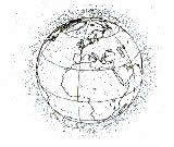
million pounds of human-made materials circling the Earth. Rings
are already forming around Earth - not the rings of rock and dust and ice
that encircle other planets, but rings of human-made orbital debris - and
their density is increasing. According to Don Kessler, a NASA scientist who
has made a career of studying space debris, "Rings are nature's way of
saying it doesn't like things in non-circular orbit out of Earth's equatorial
plane. Nature wants to tear these objects apart and reform them into either a
ring or a single object-it is just a question of when." The
North American Aerospace Defense Command (NORAD) reported in 1986 that 4488
of 6194 radar-trackable objects were orbital debris. The rest included 1582
payloads, 68 interplanetary probes, and 56 items of interplanetary probe
debris. A radar-trackable object in space is baseball size or larger, but
during hypervelocity, which begins at 3 kilometers per second, particles as
small as a paint flake can be damaging or even lethal. By the mid-1980's,
ground based telescopes made it possible for scientists to see marble-sized
pieces of orbital debris. From these observations, they concluded that the
number of debris objects was many times the number that NORAD had cataloged. The
first loss of a spacecraft part directly attributable to human-made orbital
debris occurred during the Shuttle mission of STS-7 in 1983. The crew of the
Challenger reported an impact crater on one of the orbiter's windows
significant enough to require replacement despite the fact that the window
was 5/8 inch thick and built to withstand pressures of 8600 pounds per square
inch and temperatures up to 482°C. By studying the traces found in the pitted
window, NASA determined that the damage was caused by white paint specks
about 0.2 millimeters in diameter traveling between 3 and 5 kilometers per
second. Cosmonauts
on the Soviet spacecraft Salyut 7 reported a similar window incident just
weeks later and even reported hearing the impact. The Solar Maximum Mission
satellite had been in space for fifty months when the crew of STS-41C
repaired it in space and returned to Earth with 15 square feet of the
insulation blanket and 10 square feet of aluminum louvers showing thousands
of pits and excessive wear and tear. The blanket showed thirty-two holes per
square foot and the louvers, six holes per square foot, many more than NASA
scientists expected; analysis revealed that most of the pits were caused by
paint flakes. Collisions
and breakups significantly increase the number of particles orbiting Earth,
but they differ in fragmentation and the resulting hazards. Collisions
produce smaller fragments and increased hazard. If a 10-pound mass hits a
1000 pound stage at orbital speeds, a tremendous amount of energy is released
that could result in 4 million particles and 10000 larger pieces. Breakups
caused by explosions produce fewer small fragments, which give scientists a
greater likelihood that they can learn about the causes of explosions and
thus prevent them. For example, when seven second-stage Delta rocket breakups
occurred three years after launch, scientists were able to determine that
they had been caused by unspent hypergolic fuels; this knowledge resulted in
launch changes that apparently corrected that problem.” Engagement: Day 1 Modeling
Space-Debris Accumulation Space
Debris: Is It Really That Bad? (See
Activity Sheet 1 ) The
information presented in this activity includes numbers like 4 million
pounds, 1.8 million pounds per year, and 9.5 million pounds. We have become
accustomed to reading such numbers, but few of us have an intuitive sense of
what they represent. At the beginning of the activity, students are asked to come
up with some concrete models of just what such quantities mean. They should
find it enjoyable to come up with examples like "9.5 million pounds of
pennies would fill" and other original representation. Exploration: Day 2 Modeling
the Problem: Linear Growth The
NASA predictions reported in this activity afford an excellent opportunity to
have students create and analyze simple mathematical models. Because
mathematicians strive to find the simplest model that will adequately
represent the problem, a good starting point for students is to create linear
models for the amount of accumulated space debris on the basis of the number
of pounds being added each year. In so doing, they will look at the 1990
accumulation rate of 1.8 million pounds pre year (rate of increase) and an
initial amount of 4 million pounds. If we let the years be represent by t
(with t = 1 in 1990) and the total pounds of debris by y (in units of 10^6
pounds), our linear model is y = 1.8t + 4. Similarly, if we use the rate of
.7 million pounds per year, we get y = 2.7t + 4. This result gives rise to
two new questions: (1) Where does the "eventual" 9.5 million pounds
come from? and (2)Does either model realistically describe the situation? In
this activity, it is also suggested that you make the analogy to velocity.
Because students are familiar with distance-rate-time problems, they should
be able to see that increasing the amount of debris at a constant rate is
equivalent to increasing the distance traveled when moving at a constant speed.
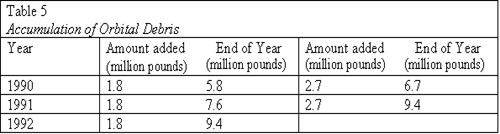
Using the two linear equations or a table, students discover that 9.5 million
pounds occur in just over three years at the first rate and in just over two
years at the second rate (see table 5).
A
good discussion should result regarding the fact that the prediction did not
specify when the 9.5 million pounds would be reached; as students will see
later, other actors must be considered when evaluating the prediction. The
students should also realize that neither model is accurate because neither
rate, 1.8 million pounds per year and 2.7 million pounds per year, applies
for the entire period from 1990 through 2000. Exploration,
continued: Day 3 Refining
the Model: Quadratic Growth Once
students realize that neither of their original attempts at a model truly
represents the situation, they should try to adjust the model to account for
the fact that neither the rate of 1.8 million pounds per year continues
throughout the period. Because scientists and mathematicians prefer to start
with a simple model and then add complexities to refine it as needed, we make
the simplest assumption to account for the changing rate of increase over the
period, namely, that the rate of adding debris increases at a constant rate
from 1.8 million pounds per year to 2.7 million pounds per year. That is, the
rate (velocity) of littering increased by 0.9 million pounds per year
achieved in equal increments of 0.09 million pounds per year each year over a
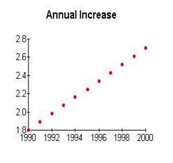
ten-year period. The students can then create a table and a graph of the rate
of "dumping" versus the year by using the data points (0, 1, 8) and
(10, 2, 7). This change of rate of dumping is given by the equation d = 0.09a
+ 1.8, where a = 0 in 1990. The increase in both the dumping rate and the
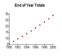
total accumulation are shown in table 6 and figure 3.
At
this point emerge a number of important concepts to explore. Although both
plots in figure 3, and those that your students generate, may appear to be
linear over the ten-year range of the initial data, extending the domain to
twenty or thirty or fifty years, as suggested on the student page, makes it
evident that the graph of the end-of-year total accumulation is, indeed, not
linear. The fact that it is quadratic can be approached from several
perspectives:
Applying
the Method of Constant Differences
The desired function is
f(x) = 0.045x2 + 1.755x + 4, where f(x) gives the amount of debris
in orbit at the end of year x and x equals 1 in 1990. Overlay this equation
on the earlier scatter plot.
Extension: Velocity-Acceleration Analogy “The
student pages compare the quadratic model for debris with the more familiar
case of constant acceleration. Students who have studied motion in a physics
class should make the connection between examples of uniformly accelerated
motion, such as a free fall, a ball rolling down an incline, or a car
accelerating at a constant rate, and the "uniform acceleration of space
dumping." With your more advanced mathematics students, you will want to
pursue the fact that the linear equation d = 0.09x + 1.8, where x is the
number of years since 1990, is the equation of the tangent to the curve y =
0.045x^2 + 1.755x + 4, the equation previously derived. That is, the first
equation is the derivative of the second. In
this section, students are likely to have the greatest difficulty
differentiating among the "rate (velocity) of littering" (e.g., 1.8
million pounds per year in 1990), the "total change in the littering
rate over then years" (i.e., an increase of 0.9 million pounds per year
between the 1990 rate of 1.8 million pounds per year and the 2000 rate of 2.7
million pounds per year), and the "rate of change (acceleration) of
littering velocity" (an increase of 0.09 million pounds per year each
year). You will need to pay special attention to these concepts. In
comparing the quadratic model, y = 0.045x^2 +1.755 + 4, with the two linear
models, y = 1.8x + 4 and y = 2.7x + 4, students will find that the graph of
the quadratic lie between the two lines. They should be able to interpret
this result in terms of what would happen if the rate of adding debris stayed
at 1.8 million pounds per year, was always 2.7 million pounds per year, or
gradually changed from 1.8 to 2.7 million pounds per year. They should also
determine when the value of the quadratic will surpass the second linear
function and recognize that thereafter the quadratic will always produce
greater values.” Exploration,
continued: Day 4 One
More Perspective: Exponential Growth The
third model proposed in this unit is an exponential one: What will happen if
the debris accumulates as a fixed percent of what is already in orbit? This
question is, of course, analogous to the familiar problem of compound
interest, and it gives an alternative context for exploring the concept of
exponential growth. It is a setting in which you will almost surely want
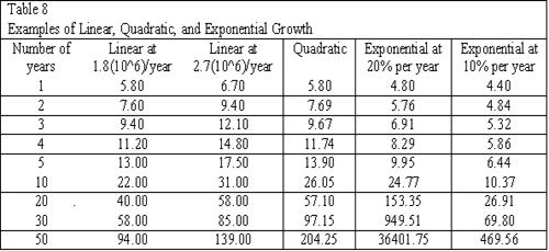
students to use a spreadsheet. The
major objective is to help students realize the impact of exponential growth.
With a spreadsheet they can hypothesize different rates of increase and
explore what would happen if debris were to be added at those rates. The
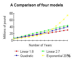
findings can be compared with the patterns of linear and quadratic growth.
Some examples are shown in table 8 and the graphs in figure 4; the amounts
are in millions of pounds.
Extension: What
Goes Up Might Come Down: Extending the Models “Students should realize, however, that not
everything in orbit stays there forever. Orbiting objects will also be pulled
back into Earth's atmosphere, where they will burn up or, on occasion, return
to Earth. To be realistic, the models that students develop should take into
account both the addition to, and the destruction of, orbital debris. We do not provide any particular data for this
section so that students will have the opportunity to form and test
hypotheses of their own. They should try modifications that assume
destruction at a fixed rate per year (linear) as well as at a fixed percent
(exponential decay). They are looking for models that might predict an
eventual decrease in the amount of orbital debris even though we assume that
NASA and others will continue to launch payloads and thereby continue to add
to the orbital debris. These open-ended investigations are designed to let
students experience the search for models that might lead to desirable
consequences - although, in reality, we may need to invent the necessary
technology to implement the model.” Putting
Your Models to Work “Finally, students are encouraged to generate
"What if" questions and to use their models to help generate
answers. Before you ask them to formulate their questions, you might want to
pose some of your own. The following are examples: What
if, at the end of 1995, we were able to stop adding to the debris and were
able to decrease the existing debris at a rate of 0.35 million pounds per
year for the next three years? What would be the total poundage remaining at
the end of 1998? What would be the percent of decrease? Note that the answers
will vary depending on what assumptions are made about the rate of increase
during the years 1990-1995. In
addition, what if, at the beginning of 1999, new technology would allow us to
improve the rate of decrease to 0.65 million pounds per year for a two-year
period? What would be the total debris remaining at the end of the century?” Modeling
Collision Effects (See
Activity Sheet 2)
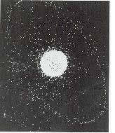
“The photo shows the
"energy flash" when a projectile launched at speeds up to 17,000
mph impacts a solid surface at the Hypervelocity Ballistic Range at NASA's
Ames Research Center, Mountain View, California. This test is used to
simulate what happens when a piece of orbital debris “This activity presents a problem of major
significance to the aerospace community: the consequences of impact at
hypervelocity. Tests done in the NASA laboratories as well as evidence from
returned spacecraft confirm the enormous damage that can be rendered by even
very small particles striking at orbital speeds. This activity introduces the
concept of kinetic energy. If your students are studying physics or physical
science, they should be familiar with this form of energy. The unit of a
joule will be less familiar, since it is a "highbred" unit and not
something for which we have everyday references. Rather than dwell on what
one joule might be, it is more useful to calculate the kinetic energy of some
everyday examples, such as a truck traveling
at highway speeds or a hard-hit ball, and then relate other energies, such as
the kinetic energy of impact from a point flake in orbit, as some multiple or
fraction of the more familiar examples. You may be surprised to discover that
a 1-gram paint chip traveling at orbital speed has nearly 1/10 the kinetic
energy of a 3500-pound truck moving at 60 miles per hour and that a 350-pound
satellite at orbital speed has 10000 times the kinetic energy of the truck. In this section, students must pay close attention
to units, and you will want to be sure that they recognize that to be
meaningful, their calculations of such quantities as mass, velocity, and
energy must be expressed in appropriate units. You will note that the units
used in the activity are mixed - pounds, kilograms, grams, miles per hour,
kilometers per second, and so on - because they are the units commonly used
in measuring the associated phenomena. This situation is realistic, and with
spreadsheets and calculators, conversions should pose no particular problems.
Cautious attention to units, however, is required. Also, some measurements
are left for students to find or approximate, such as the mass of a baseball
or the velocity at which it may be hit. Sports enthusiasts sometimes carry
this sort of information in their heads; others may prefer to use data from
their own sports exploits; still others will look up the data in a book of
sports statistics. Again, the purpose of the activity is to foster
open-ended investigation and discussion of the relative effects of the linear
factor (mass) compared with the quadratic component (velocity). We are less
concerned with precise answers to particular questions than we are with the
larger concept of how these functions behave.” Modeling
Collision Probability (See
Activity Sheet 3 ) “Throughout this unit, we have looked at enormous
quantities - millions of pounds - of debris. But we have not yet related
those quantities to the vastness of space, even the relatively "close
fitting" sphere in which payloads orbit Earth. This activity has
students calculate the volume of a "shell" 200 kilometers thick
extending from an altitude of 200 to 400 kilometers above Earth - a volume of
just over 1.1(1011) cubic kilometers. If we assume that 4 million
pounds (1.8 million kilograms) of debris are evenly distributed throughout
this volume, we find the density of debris to be on the order of 1.6(10-5)
kilogram, or 0.016 gram, per cubic kilometer. In the activity, we assume that the debris has the
density of aluminum, 2.7 grams per cubic centimeter. By making this
assumption, we can estimate that the 0.016 gram per cubic kilometer
represents approximately 0.006 cubic centimeter of debris per cubic kilometer
of the shell. The probability of hitting any of that debris is the ratio of
the volume of debris to the volume of the shell; hence, we can estimate the
probability of hitting the debris to be on the order of 6(10-12).
Removing the simplifying assumption of a 200-kilometer thick shell does not
change the order of magnitude of the probability.” |
|||||||||||||||||||||||||||||||||||||||||||||||||||||||||||||||||||||||||||||||||||||||||||||||||||||||||||||||||||||||||||||||||||||||||||

References
- Originally
Adapted from Modeling Orbital Debris Problems in Mission Mathematics, Linking Aerospace and the NCTM
Standards, 9-12, a NASA/NCTM project, NCTM 1997.
- Revised
and reformatted by Ellen Lukasik,
- Images
from: http://spaceflight.nasa.gov/gallery/images/mars/marsvehicles/med/s95_01414.jpg
and http://spaceflight.nasa.gov/gallery/images/mars/lunarvehicles/med/s83_28321.jpg
 Name
______________________________
Name
______________________________
Modeling Orbital Debris Problems
Space Debris: Is It Really That Bad?
Student Activity Sheet 1
One problem with which NASA and space scientists from other countries must deal is the accumulation of space debris in orbit around Earth. Such debris includes payloads that are no longer operating; spent stages of rockets, assorted parts and lost tools; debris from the breakup of larger objects or from collisions between objects; and countless small pieces, such as flakes of paint and even smaller objects. Because bodies in Earth orbit travel at approximately 17500 miles per hour, a collision with even a tiny object can have catastrophic effects. In 1990, scientists estimated that a total of 4 million pounds of debris was in Earth orbit. They also estimated that at that time, we were adding 1.8 million pounds per year to the already serious problem, which in a few years would result in 9.5 million pounds of orbital debris. The 1990 prediction also stated that the amount of debris being added was anticipated to increase to a rate of 2.7 million pounds per year by the year 2000.
Activity
1
1. How much is 4 million pounds of anything?
Or 9.5 million?
Give at least three concrete examples that would help another person get a sense of how much millions of pounds of debris is. For example, finish the following sentence.
A total of 9.5 million pounds of pennies would fill __________________.
 Modeling the
Problem: Linear Growth
Modeling the
Problem: Linear Growth
The problem of determining the amount of debris in space and the anticipated rate of increase of such matter is not one that can be solved directly. We cannot locate, count, and weigh all objects in orbit. Nor can we predict with assurance when two of them will collide. Instead, we must rely on mathematical models to help us represent the problems and identify trends and expected outcomes. In these activities, you will create and compare various mathematical models to help you investigate some of the questions raised by the proliferation of orbital debris. These models are greatly simplified in their assumptions so that you can investigate them with calculators, spreadsheets, and graphing utilities, but they provide insight into the process of mathematical modeling and its importance.
Activity 2
1.
When creating models, mathematicians favor the simplest model that will account
for the phenomena in question. Generally, a linear model gives the simplest
case. So, using the reported 1990 rate of increase of 1.8 million pounds per
year and assuming 4 million pounds of existing debris at the beginning of 1990,
write a linear model to predict the number of pounds of orbital debris at the
end of any given year, t. Assume that t = 1 represents 1990.
2. Write a second linear model using the predicted 2.7 million pounds
per year rate of increase and the initial 4 million pounds for 1909.
3. Evaluate each model for several years to determine the year in which the predicted 9.5 million pounds of accumulated debris would occur:
With the first model: ____________________
With the second model: __________________
4. When a vehicle travels at a constant rate, r, for a length of time, t, the distance traveled by the vehicle is modeled by a linear function. Compare the familiar linear model for distance-rate-time with your linear models for accumulating space debris. Why can we refer to your linear models as "constant-velocity models for amassing space debris"?
5. Do you think that either of your linear models accurately represents that situation of escalating amounts of space debris as described in the original paragraph? Why or why not?
Refining the Model: Quadratic Growth
Does either rate, 1.8 million pounds per year or 2.7 million pounds per year, tell us how much debris is building up between 1990 and 2000? Which rate of increase should we use? Obviously the amount being added each year is changing during this period, but by how much each year? The problem is one of acceleration, no constant velocity, so we need to adjust our model.
Again, let's make the simplest assumption: the rate at which we are adding debris increases at a constant rate from 1.8 million pounds per year in 1990 to 2.7 million pounds per year in 2000. This change means that over the ten-year period from the end of 1990 through 2000, the rate (velocity) of littering will increase by 0.9 million pounds per year (2.7 - 1.8 = 0.9), and we are making the assumption that this increase is achieved in equal annual increments of 0.09 million pounds per year in each year of the decade.
Activity 3
1. Complete the following table to show the amount of debris added each year and the total amount in orbit at the end of the year.
2. Since we assumed that the increase in the velocity of littering was achieved in equal annual increments, you can write a linear equation that describes the increase in the amount of debris being added each year (i.e, the increase in the annual velocity of littering as a function of the number of years since 1990. In this case, we let a = 0 in 1990 because we are assuming that the 1990 rate of 1.8 million pounds per year is our baseline rate. Then d = f (a) represents the rate of littering a years after 1990.
2.
The situation described in your equation, where the rate of increase of litter
is itself increasing at a constant rate, is analogous to a vehicle that
accelerates at a constant rate from an initial velocity, v0, to a final
velocity, vf. Use the data generated in the foregoing
table to create a scatterplot of the total number of pounds of orbital debris
that have accumulated relative to the year. You graph should cover the period
from 1990 through 2000.
3.
Fit a line to you data and decide whether the accumulation of debris appears to
be linear. Write your conclusion and describe the evidence on which you based
your decision.
4. Using a graphing calculator or computer graphing program, calculate the linear-regression equation for these data.
Do your calculations support a linear relationship? Explain.
How does this line compare with the line that you fitted manually?
5. Next generate a quadratic-regression equation for the same data. Write the quadratic-regression model here:
How well does this equation fit the data compared with the linear approximation?
6. Compare your quadratic-regression equation with the two linear-regression equations that you developed earlier.
7.
In each case, use your models to predict the accumulation of debris after
twenty years, thirty years, and fifty years. Describe the behavior of the
linear model versus the quadratic model over time.
8.
For the period from 1990 to 2000, the graph of the quadratic model lies between
the graphs of the two linear models. Explain why this result is reasonable.
Will the quadratic graph always lie between the two linear graphs? Explain.
9.
Explain why the quadratic model for the debris problem can be described as a
"uniform acceleration" model.
One More Perspective:
Exponential Growth
So far, you have looked at
two models, a "constant velocity" linear model and a "uniformly
accelerated" quadratic model. Let's look at one more model.
Activity 4
1. Suppose that the amount of litter added each year
grew not by a fixed number of pounds but by a fixed percent of the amount
already in space - a situation analogous to an investment of money with
interest compounded annually. For example, what would happen to the original 4
million pounds if the litter added each year was 20 percent of the amount
already in orbit? Complete the following table to determine the amount of
debris that would accumulate over the period from 1990 to 2000. A spreadsheet
is recommended for this activity.
2. Write an exponential
model to describe the growth of the original 4 million pounds of debris over
the years:
3. Use your model to predict the amount of debris that would accumulate in
twenty years, thirty years, and fifty years.
4. Economists use what is referred to as the
"rules of 72" to predict how long it will take an amount of money to
double if it is invested at a rate of R percent compounded annually. According
to the rules of 72, the doubling time, D, is given by the equation.
D = 72/R
Use the rule of 72 to predict how long it will take
for the amount of debris to
Double if littering compounds at the rate of 20 percent per year. How long
will it take for the original 4 million pounds to increase to 32 million
pounds?
Do the data in your table agree with those
calculations?
5. If the growth of space debris was following an
exponential model and concern arose that it would take only twelve years to
double the amount of space debris, what must the annual percent increase in
debris have been to result in this doubling time of twelve years?

What Goes Up Might Come Down: Extending the Models
Activity 5
All
the models you have developed thus far assume that the additional every year
some of the debris slows down enough to re-enter the atmosphere where it burns
up or, on rare occasions,
returns to Earth. Assume for the moment that 10 percent of the debris in orbit
at the beginning of any year will be destroyed during that year.
1.
Modify you linear, quadratic, and exponential models to account for the
situation in which additional debris is being added each year while 10 percent
of what was already in orbit is being destroyed.
2.
In which case - linear, quadratic, or exponential - does the assumption of a 10
percent re-entry rate have the greatest effect?
3.
Assume the same rates of adding debris as you did you when you generated the
models, but try different rates of annual destruction of orbital debris. In
each situation, does a destruction rate exist that will result in a net
decrease in orbital debris despite the fact that additional debris is being
added?
4. What might be some advantages of knowing if such a rate is possible?
Putting Your Models to Work
The power of mathematical models comes from their ability to enable us to ask "What if?" questions. An earlier question is an example: What if we could increase the rate at which orbital debris is destroyed? Other questions might include these: What if we decrease the rate at which we are adding debris and find a way to increase the rate at which existing debris is destroyed? Such questions lead to open-ended investigations using mathematical models.
Activity 6
1. Working with a partner or a small group, generate two or three specific questions that you would like to investigate.
1. What if…
2. What if…
3. What if …
2. Describe a plan for investigating your questions using spreadsheets, graphing utilities, or other appropriate technology.